Real estate cohort analysis


After in the last post we looked how to get the data, now we are going to start analyzing it. The first question we are interested in is how quickly do houses sell. We don't have access to actual contracts, so we will use a proxy to measure this: how long is an advertisment for a house still displayed. We are going to estimate that this is roughly the time it takes to sell a house.
We will do a cohort analysis, where each cohort will be composed of ads that were shown for the first time on that day and we will track what percentage of those ads is still shown as days pass.
To do this, we will need to gather data for some time, running our scraper daily. I did for almost three months now. I forgot to run it on some days (and I have an item on my todo list to automate this for almost three months now), so I have about 75 entry points.
Let's start by reading in the data. We are going to use Pandas for this, because it has support for the JSON lines format.
import pandas as pd
import matplotlib.pyplot as plt
import glob
import seaborn as sns
sns.set(style='white')

data = pd.concat([pd.read_json(f) for f in glob.glob("../data/houses*.jl")],
        ignore_index=True)
data = data.drop(columns=["adaugat_la", "Compartimentare", "text"])
data["nr_anunt"] = data["nr_anunt"].map(lambda x: x[0] if type(x) == list else x)
First we do some imports and set some graph plotting settings. Then we read all the data into a big Pandas dataframe and we drop some of the columns we don't need for our analysis right now and we fix some issues with the nr_anuntcolumn (sometimes it's a list).
data.set_index('nr_anunt', inplace=True)

data['CohortGroup'] = data.groupby(level=0)['date'].min()
data.reset_index(inplace=True)
We reset the index, to be according to the nr_anunt column, which is the ID of each ad, so it identifies each ad uniquely. Then we create a new column, by grouping by the index and taking the minimum out of each group. When we group by the index, it means that each group will contain each scraping of an ad, taken on different days. By taking the minimum of the date, we get the first time we saw the ad.
grouped = data.groupby(["CohortGroup", "date"])
cohorts = grouped.agg({'nr_anunt': pd.Series.nunique})

cohorts.head()| CohortGroup | date | count |
|---|---|---|
| 2018-02-07 | 2018-02-07 | 2551 |
| 2018-02-08 | 2461 | |
| 2018-02-09 | 2390 | |
| 2018-02-10 | 2345 | |
| 2018-02-11 | 2300 |
Then we group the data again, this time by the CohortGroup and by the date we saw the ad. The first grouping means we put in one group all the ads that showed up the first time on a certain day, and then we group again by every subsequent day when we saw them. On these groups, we aggregate by the number of unique IDs we see, which will give us the size of our cohorts on each day.
exp = pd.DataFrame(cohorts.to_records())

exp["CohortPeriod"] = exp["date"] - exp["CohortGroup"]
exp.set_index(["CohortGroup", "CohortPeriod"], inplace=True)
exp.head()| CohortGroup CohortPeriod | CohortPeriod | date | nr_anunt |
|---|---|---|---|
| 2018-02-07 | 0 days | 2018-02-07 | 2551 |
| 1 days | 2018-02-08 | 2461 | |
| 2 days | 2018-02-09 | 2390 | |
| 3 days | 2018-02-10 | 2345 | |
| 4 days | 2018-02-11 | 2300 |
Until now, we have absolute dates, which we can't compare between cohorts. If one cohort started in March, and the other one in April, of course they will have different behaviours in April (one being right at the beginning and the other one one month in). So we want to convert to relative dates, by substracting the date of the scraping of the ad and the first time we saw the ad. Because my Pandas-fu is not that good, I didn't find another solution to this other than expand the index to columns again. Then I did the substraction and reindexed everything, this time by the CohortGroup (so first day an ad showed up) and CohortPeriod (how many days have passed since then).
cohort_group_size = exp["nr_anunt"].groupby(level=0).first()
retention = exp["nr_anunt"].unstack(0).divide(cohort_group_size, axis=1)
retention.head()| Cohort Group CohortPeriod | 2018-02-07 | 2018-02-08 | 2018-02-09 | 2018-02-10 | 2018-02-11 |
|---|---|---|---|---|---|
| 0 days | 1.000000 | 1.000000 | 1.000000 | 1.00000 | 1.000000 |
| 1 days | 0.964720 | 0.921569 | 0.941176 | 1.00000 | 0.955882 |
| 2 days | 0.936887 | 0.901961 | 0.862745 | 0.93750 | 0.852941 |
| 3 days | 0.919247 | 0.901961 | 0.862745 | 0.90625 | 0.852941 |
| 4 days | 0.901607 | 0.882353 | 0.862745 | 0.87500 | 0.794118 |
We are now ready to calculate retention. We want percentages, not absolute values, so we first look at the size of each cohort on the first day. Then we pivot the dataframe, so that on the rows we get CohortPeriod and on the columns we get CohortGroups (that's what unstack does) and divide with the size of the cohorts, column-wise.
And then we plot what we got. First, we can do a line chart:
retention.plot(figsize=(15,10))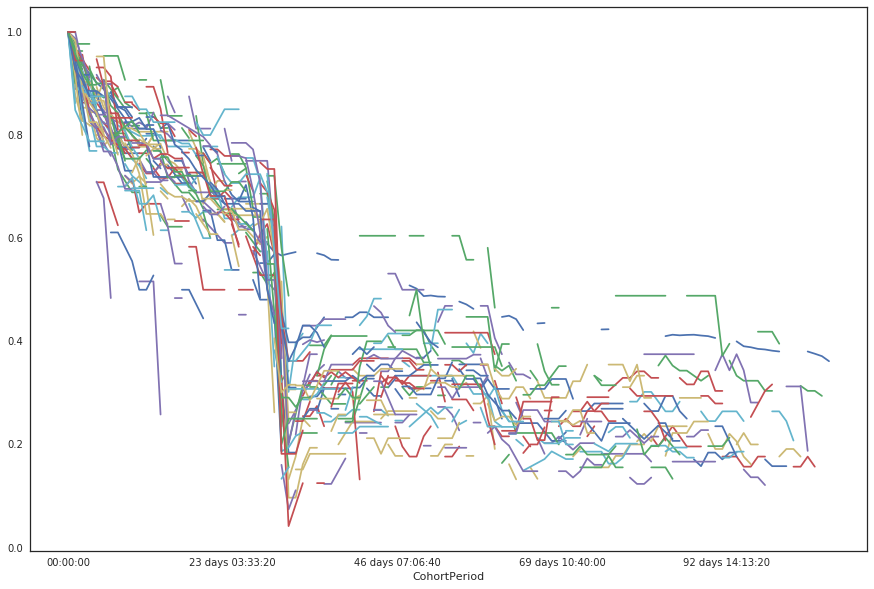
And then a nice heatmap:
sns.heatmap(retention.T, fmt='.0%', )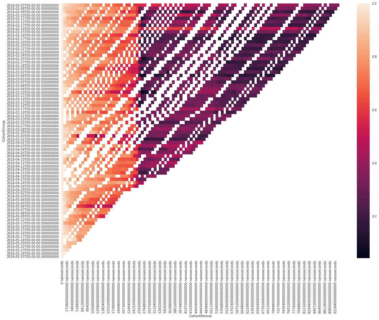
From looking at these two charts, we see that after about one month, 60% of the ads are still available, but then, there is a big cliff and it jumps down to below 30%. However, then it climbs back up, to around 40% and then stabilizes around 30%.
My hypothesis is that after the first month, the ads are taken offline by an automated system, for inactivity and that's why you have a big drop. Some people reactivate the ads, which leads to the rebounce and then ads organically go away, as the underlying real estate is no longer available.
In conclusion, you don't need to hurry too much when buying houses in Oradea: you easily have at least two weeks for 80% of the cases, after an ad shows up, and up to a month in 60% of the cases.